Контрольная работа: Endogenous Cycle Models

Контрольная работа: Endogenous Cycle Models

Contents

Introduction

1. Endogenous Cycle Models: Kaldor's Non-Linear Cycle

Conclusion

Literature

Introduction

The multiplier-accelerator structures reviewed above have linear dynamic structures. As a result, cycles are generated and maintained only by structurally unstable parameter values (Samuelson) or dampened dynamics with continuous exogenous shocks (Frisch-Slutsky) or exogenously-constrained explosive dynamics (Hicks). As a result, early Keynesian linear multiplier-accelerator fall dangerously close to an "untheoretical" explanation of the cycle - precisely what the original Oxbridge research programme was designed to avoid.

However, linear structures are often adopted because they are simple and the results they yield are simple. But simplicity is sometimes more a vice than a virtue - particularly in the case of macrodynamics and economic fluctuations. It is not only unrealistic to assume linearity, but the very phenomena that we are out to uncover, the formation of cycles and fluctuations, becomes relegated to the "untheory" of exogenous shocks, ceilings, floors, etc. The contention of Lowe (1926) and many Keynesian writers is that theories of fluctuations ought really to explain how fluctuations arise endogenously from a working system otherwise (paraphrasing Lowe's title), how is business cycle theory possible at all?

As a result, many economists have insisted that non-linear structures should be employed instead. Why interest ourselves with non-linear dynamics? As one famous scientist answered, for the same reason we are interested in "non-elephant animals". In short, non-linear dynamical structures are clearly the more general and common case and restricting attention to linear structures not only unrealistically limits the scope of analysis, it also limits the type of dynamics that are possible.

1. Endogenous Cycle Models: Kaldor's Non-Linear Cycle

One of the most interesting theories of business cycles in the Keynesian vein is that expounded in a pioneering article by Nicholas Kaldor (1940). It is distinguishable from most other contemporary treatments since it utilizes non-linear functions, which produce endogenous cycles, rather than the linear multiplier-accelerator kind which rely largely on exogenous factors to maintain regular cycles. We shall follow Kaldor's simple argument and then proceed to analyze Kaldor in the light of the rigorous treatment given to it by Chang and Smyth (1971) and Varian (1979).

What prompted Kaldor's innovation? Besides the influence of Keynes (1936) and Kalecki (1937), in his extremely readable article, Kaldor proposed that the treatment of savings and investment as linear curves simply does not correspond to empirical reality. In (Harrodian version of) Keynesian theory, investment and savings are both positive functions of output (income). The savings relationship is cemented by the income-expenditure theory of Keynes:

S = (1-c) Y

whereas investment is positively related to income via an accelerator-like relationship, (which, in Kaldor, is related to the level rather than the change in income):

I = vY

where v, the Harrod-Kaldor accelerator coefficient, is merely the capital-output ratio. Over these two relationships, Kaldor superimposed Keynes's multiplier theory: namely, that output changes to clear the goods market. Thus, if there is excess goods demand (which translates to saying that investment exceeds savings, I > S), then output rises (dY/dt > 0), whereas if there is excess goods supply (which translates to savings exceeding investment, I < S), then output falls.

The implications of linearity can be visualized in Figure 1, where we draw two positively-sloped linear I and S curves. To economize on space, we place two separate sets of curves in the same diagram. In the left part of Figure 1, the slope of the savings function is larger than that of the investment function. Where they intersect (I = S) is the equilibrium Y*. As we can note, left of Y*, investment is greater than savings (I > S), hence output will increase by the multiplier dynamic. Right of point Y*, savings is greater than investment (I < S), hence output will fall. Thus, the equilibrium point Y* is stable.

In the right side of Figure 1, we see linear S and I functions again, but this time, the slope of the investment curve is greater than that of the savings curve. Where they intersect, Y*, investment equals savings (I = S) and we have equilibrium. However, note that left of the equilibrium Y*, savings are greater than investment (I < S), thus output will contract and we will move away from Y*. In contrast, right of Y*, investment is greater than savings (I > S), so output will increase and move further to the right of Y*. Thus, equilibrium Y* is unstable.

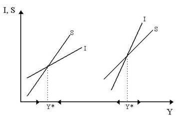
Fig.1 - Savings, Investment and Output Adjustment

Both exclusive cases, complete stability and complete instability, are implied by linear I and S curves in figure 1, are incompatible with the empirical reality of cycles and fluctuations. Hence, Kaldor concluded, it might be sensible to assume that the S and I curves are non-linear. In general, he assumed I = I (Y, K) and S = S (Y, K), where investment and savings are non-linear functions of income and capital as in the Figure 2 below.

We shall focus the relationship with income first. The logic Kaldor (1940) gave for this is quite simple.

The non-linear investment curve, shown in Figure 2 can be explained by simply recognizing that the rate of investment will be quite low at extreme output levels. Why? Well, at low output levels (e. g. at YA), there is so much excess capacity that any increase in aggregate demand will induce very little extra investment.

The extra demand can be accomodated by existing capacity, so the rate of investment is low. In contrast, at high rates of output, such as YC, Wicksellian problems set in. In other words, with such high levels of output and demand, the cost of expanding capacity is also increasing, capital goods industries are supply-constrained and thus demand a higher price from entrepreneurs for producing an extra unit of capital. In addition, the best investment projects have probably all already been undertaken at this point, so that the only projects left are low-yielding and simply might not be worth the effort for the entrepreneur.

Thus, the rate of investment will also be relatively low. At output levels between YA and YC (e. g. at YB), the rate of investment is higher. Thus, the non-linearity of the I curve is reasonably justified.

What about the non-linear savings curve, S? As shown in Figure 2, it is assumed by Kaldor that savings rates are high at extreme levels of output. At low levels of output (YA), income is so low that savings are the first to be cut by individuals in their household decisions.

Therefore, at this point, the rate of saving (or rather, in this context, the rate of dissaving) is extremely high. Slight improvements in income, however, are not all consumed (perhaps by custom or precaution), but rather much of it is saved.

In contrast, at high levels of output, YC, income is so high that the consumer is effectively saturated. Consequently, he will save a far greater portion of his income - thus, at points like YC, the savings rate is quite high.

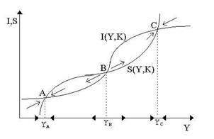
Fig.2 - Non-Linear Investment and Savings

With the non-linearity of I and S justified, Kaldor (1940) proceeded to analyze cyclical behavior by superimposing the I and S curves (as in Figure 2). As we can see, there are three points of intersection (A, B and C) where savings equals investment (I = S). Let us consider each individually. Left of point A, investment is greater than savings hence, by the multiplier, Y increases to YA; to the right of point A, savings is greater than investment (hence Y decreases to YA). Consequently, it is easy to note that A (and YA) is a stable point. The same analysis applies to the points to the right and left of YC, hence C (and YC) is also a stable point.

Intersection point B (at YB) in Figure 2 is the odd one. Left of B, savings exceeds investment (so Y falls left of YB) and right of B, investment exceeds savings (so Y increases right of YB). Thus, B is an unstable point. Consequently, then, we are faced with two stable equilibria (A and C) and an unstable equilibrium (B). How can this explain cyclical phenomenon? If we are at A, we stay at A. If we are at C, we stay at C. If we are at B, we will move either to A or C with a slight displacement. However, no cycles are apparent.

The clincher in Kaldor's system is the phenomenon of capital accumulation at a given point in time. After all, as Kaldor reminds us, investment and savings functions are short term. At a high stable level of output, such as that at point YC in the figure above, if investment is happening, the stock of capital is increasing. As capital stock increases, there are some substantial changes in the I and S curves. In the first instance, as capital stock increases, the return or marginal productivity of capital declines. Thus, it is not unreasonable to assume that investment will fall over time. Thus, it is acceptable that dI/dK < 0, i. e. the I curve falls.

However, as capital goods become more available, a greater proportion of production can be dedicated to the production of consumer goods. As consumer goods themselves increase in number, the prices of consumer goods decline. For the individual consumer, this phenomenon is significant since it implies that less income is required to purchase the same amount of goods as before. Consequently, there will be more income left over to be saved. Thus, it is also not unreasonable to suspect that the savings curve, S, will gradually move upwards, i. e. dS/dK > 0. This is illustrated in Figure 3.

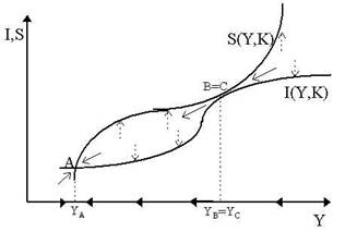
Fig.3 - Capital Accumulation and Gravitation of Investment and Savings Curves

So, we can see the story by visualizing the move from Figure 2 to Figure 3. Starting from our (old) YC, as I (Y, K) moves down and S (Y, K) moves down, point B will gradually move from its original position in the middle towards C (i. e. YB will move right) while point C moves towards B (YC moves left). As shown in Figure 3, as time progresses, and the investment and savings curves continue on their migration induced by capital accumulation, and B and C approximate each other, we will reach a situation where B and C meet at YB = YB and the S and I curves are tangential to each other. Notice that at this point in time, C is no longer stable - left and right of point C, savings exceeds investment, thus output must fall - and indeed will fall catastrophically from YB = YC to the only stable point in the system: namely, point A at YA.

At YA, we are again at a stable, short-run equilibrium. However, as in the earlier case, the S and I curves are not going to remain unchanged. In fact, they will move in the opposite direction. As investment is reigned back, there might not even be enough to cover replacement.

Thus, previous investment projects which were running on existing capital will disappear with depreciation. The usefulness (i. e. productivity) of the projects, however, remains. Thus, the projects reemerge as "new" opportunities. In simplest terms, with capital decumulation, the return to capital increases and hence investment becomes more attractive, so that the I curve will shift upwards (see Figure 4).

Similarly, as capital is decumulated, consumer industries will disappear, prices rise and hence real income (purchasing power) per head declines so that, to keep a given level of real consumption, savings must decline. So, the S curve falls. Ultimately, as time progresses and the curves keep shifting, as shown in Figure 4, until we will reach another tangency between S and I analogous to the one before. Here, points B and A merge at YA = YB and the system becomes unstable so that the only stable point left is C. Hence, there will be a catastrophic rise in production from YA to YC.

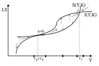
Fig.4 - Capital Decumulation and Gravitation

Thus, we can begin to see some cyclical phenomenon in action. YA and YC are both short-term equilibrium levels of output. However, neither of them, in the long-term, is stable. Consequently, as time progresses, we will be alternating between output levels near the lower end (around YA) and output levels near the higher end (around YC). Moving from YA to YC and back to YA and so on is an inexorable phenomenon. In simplest terms, it is Kaldor's trade cycle.

W. W. Chang and D. J. Smyth (1971) and Hal Varian (1979) translated Kaldor's trade cycle model into more rigorous context: the former into a limit cycle and the latter into catastrophe theory. Output, as we saw via the theory of the multiplier, responds to the difference between savings and investment. Thus:

dY/dt = a (I - S)

where a is the "speed" by which output responds to excess investment. If I > S, dY/dt > 0. If I < S, dY/dt < 0. Now both savings and investment are positive (non-linear) functions of income and capital, hence I = I (K, Y) and S = S (K, Y) where dI/dY= IY > 0 and dS/dY = SY > 0 while dI/dK = IK < 0 and dS/dK = SK > 0, for the reasons explained before. At any of the three intersection points, YA, YB and YC, savings are equal to investment (I - S = 0).

We are faced basically with two differential equations:

dY/dt = a [I (K,Y) - S (K,Y)], dK/dt = I (K, Y)

To examine the local dynamics, let us linearize these equations around an equilibrium (Y*, K*) and restate them in a matrix system:

the Jacobian matrix of first derivatives evaluated locally at equilibrium (Y*, K*), call it A, has determinant:

|A| = a (IY - SY) IK - a (IK - SK) IY, = a (SKIY - IKSY)

where, since IK < 0 and SK, SY, IY > 0 then |A| > 0, thus we have regular (non-saddlepoint) dynamics. To examine local stability, the trace is simply:

tr A = a (IY - SY) + IK

whose sign, obviously, will depend upon the sign of (IY - SY). Now, examine the earlier Figures 3 and 4 again. Notice around the extreme areas, i. e. around YA and YC, the slope of the savings function is greater than the slope of the investment function, i. e. dS/dY > dI/dY or, in other words, IY - SY < 0. In contrast, around the middle areas (around YB) the slope of the savings function is less than the slope of the investment function, thus IY - SY > 0. Thus, assuming Ik is sufficiently small, the trace of the matrix will be positive around the middle area (around YB), thus equilibrium B is locally unstable, whereas around the extremes (YA and YC), the trace will be negative, thus equilibrium A and C are locally stable. This is as we expected from the earlier diagrams.

To obtain the phase diagram in Figure 5, we must obtain the isoclines dY/dt = 0 and dK/dt = 0 by evaluating each differential equation at steady state. When dY/dt = 0, note that a [I (Y, K) - S (Y, K)] = 0, then using the implicit function theorem:

dK/dY|dY/dt = 0 = - (IY - SY) / (IK - SK)

Now, we know from before that Ik < 0 and Sk > 0, thus the denominator (Ik - Sk) < 0 for certain. The shape of the isocline for dY/dt = 0, thus, depends upon the value of (Iy - Sy). As we claimed earlier, for extreme values of Y (around YA and YC), we had (IY - Sy) < 0, thus dK/dY|Y < 0, i. e. the isocline is negatively shaped. However, around middle values of Y (around YB), we had (IY - SY) > 0, thus dK/dY|Y > 0, i. e. the isocline is positively shaped. This is shown in Figure 5.

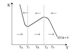
Fig.5 - Isokine for dY/dt = 0

From Figure 5, we see that at low values of Y (below Y1) and high values of Y (above Y2), the isokine is negatively-sloped - this corresponds to the areas in our earlier diagrams where the savings function was steeper than the investment function (e. g. around YA and YC). However, between Y1 and Y2, the isokine is positively-sloped - which corresponds to the areas where investment is steeper than savings (around YB in our earlier diagrams).

The off-isokine dynamics are easy, namely differentiating the differential equation dY/dt for K:

d (dY/dt) /dK = a [IK - SK] < 0

as IK < 0 and SK > 0. Thus, above the isokine, dY/dt < 0, so output falls whereas below the isokine, dY/dt > 0, so output rises. The directional arrows indicate these tendencies. We can already get a flavor of Kaldor's trade cycle from Figure 6. Remember that our earlier Kaldorian diagrams were drawn for a particular level of capital, K. Thus, as we see in Figure 6, for a given level of K0, we can find the corresponding equilibria (YA, YB, YC) at the intersection between the isokine and the level line K0. However, suppose we start at point C so that K begins to rise: notice that when K0 rises to K2, the points YC and YB begin to move together and finally "merge" at the critical point D (which corresponds to our old B=C) at point Y2. The underlying dynamic (represented by the phase arrows) implies that point D is completely unstable so there will be a catastrophic jump from D to the lower equilibrium E (which is where A moved to as K rose from K0 to K2). Notice that during this catastrophic fall in output is driven solely by the fast multiplier dynamic - the slower-moving capital dynamic is inoperative as, in moving from D to E, capital is constant at K2.

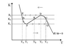
Figure 6 - Dynamics of the Kaldor Cycle

The rest of the story then follows in reverse. At E in Figure 6, we are at a pretty low output level and thus capital decumulates and so K declines from K2 past K0 and then on towards K1. In the meantime, our lower two equilibrium begin to move towards each other and A and B meet and merge at point F at Y1 (equivalent to our old A=B). Note that the stability arrows in Figure 6 are such that now we must have a catastrophic jump in output from F to point G (the high equilibrium to which point C moved to as capital fell from K2 to K1). From G, the process then begins again as capital rises at high output levels from K1 to K0 and onto K2.

The output cycle that can be traced out from the arrows drawn in Figure 6 (from slow movement from G to C to D then catastrophic jump to E then slow movement from E to A to F then catastrophic jump to G, etc) is Kaldor's trade cycle: output thus fluctuates over time between the boundaries imposed by the extreme points E (lower bound) and G (upper bound). Notice that the cycle is completely endogenous: no exogenous shocks, ceilings, floors, structurally unstable parameter values or ratchets are necessary to obtain constant cycles. The non-linearity of the curves, which are economically-justified and not exceptional, is more than sufficient to generate endogenous cycles.

This version of Kaldor's model is derived a bit more formally in Varian (1979) using catastrophe theory. However, we can also use regular non-linear dynamical theory, which makes no assumptions about the relative speeds of the dynamics, to obtain a cycle from the Kaldor model - and this is what Chang and Smyth (1971) do. We have already derived the isokine dY/dt = 0, so to get the full story, we need the dK/dt = 0 isokine. This is simple. dK/dt = I (Y, K), thus at steady-state, dK/dt = 0 = I (Y, K) so the isokine has slope:

dK/dY|K = - IY/IK > 0

as IY < 0 and IK > 0. Thus, the dK/dt = 0 isokine is positive sloped. We have superimposed it on the other isokine in Figure 7. For the off-isokine dynamics, note that:

d (dK/dt) /dY = IY > 0

so that the directional arrows drawn in for the dK/dt = 0 isokine imply that to the left of it, dK/dt < 0 (capital falls) whereas to the right, dK/dt > 0 (capital rises). In the figure below, we have superimposed the isokines for the whole system. As is obvious, the global equilibrium, where dK/dt = dY/dt = 0, is at K* and Y* (point E). Now, as we showed earlier, the trace of the system, tr A, is positive around point E, thus we know that the global equilibrium is locally unstable - as is shown in Figure 7 by the unstable trajectory that emerges when we move slightly off the equilibrium point E. .

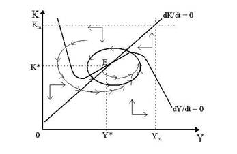
Fig.7 - Kaldor's Trade Cycle

However, notice that the system as a whole is "stable": when we draw a "box" around the diagram by imposing upper boundaries Km and Ym in Figure 7 and letting the axis act as lower boundaries, then the directional phase arrows around the boundaries of the box indicate that we do not get out of the confines of this box - any trajectory which enters the "box" will not leave it. Indeed, from the distant boundaries, it almost seems as if we are moving towards the global equilibrium (K*, Y*). Thus, while the equilibrium (K*, Y*) is locally unstable, we are still confined within this "box". Note that we are assuming complex roots to obtain stable and unstable focal dynamics as opposed to simply monotonic ones.

In fact, these three conditions - complex roots, locally unstable equilibrium and a "confining box" - are all that is necessary to fulfill the Poincarй-Bendixson Theorem on the existence of a dynamic "limit cycle". This limit cycle is shown by the thick black circle in Figure 7 (not perfectly drawn) orbiting around the equilibrium. Any trajectory that begins within the circle created by the limit cycle will be explosive and move out towards the cycle. In contrast, any trajectory that begins outside the circle will be dampened and move in towards it. Two such trajectories are shown in Figure 7. Thus, the limit cycle "attracts" all dynamic trajectories to itself and once a trajectory confluences with the limit cycle, it proceeds to follow the orbit of the limit cycle forever (as shown by the directional arrows on the cycle).

In essence, then, all trajectories are "stable", but we are not speaking of a stable path towards a point (such as an equilibrium) but rather of a stable path towards another path, i. e. the limit cycle. This is the limit cycle version of the Kaldor trade cycle. For details on this version of the Kaldor model and more general non-linear dynamics, particularly on Poincarй-Bendixson and, more generally, the Hopf-Bifurcation necessary to yield dynamic limit cycles, consult Chang and Smith (1971), Gabisch and Lorenz (1987), Lorenz (1989) and Rosser (1991).

Conclusion

Beyond the fact that these pioneers of non-linear dynamic systems in economics were all Keynesians, there is a natural fellowship between non-linear dynamics and Keynesian cycle theory: namely, that non-linear systems, in contrast to linear systems, are far more capable of yielding regular endogenous macrofluctuations. This implies that fluctuations are the outcome and indeed an integral part of a working economy. As this concept was central to Keynes's (1936) static theory, it is no surprise that Oxbridge researchers insist on endogenous cycles as a way of extending it into a dynamic context. In contrast, Neoclassical theory seems to be more apt to consider equilibrium as opposed to fluctuations as the central feature of a working economy - and thus prefer to conceive of "fluctuations" as the results of erratic displacements or aberrations from a working economy. The Neoclassical concept of the economy, thus, is perfectly compatible with linear systems; the Keynesian concept of endogenous cycles, however, seems to require non-linear structures.

Literature

1.  Dornbusch R. и др. Macroeconomics/ R. Dornbusch, S. Fischer, R. Startz. - 8th ed. - Boston etc.: Irwin: McGraw-Hill, 2007.

2.  McConnel C. R., Brue S. L. Economics: Principles, Problems and Policies. - 14 th ed. - Boston etc.: Irwin: McGraw-Hill, 2001.

3.  Speegle R., Giesecke W. Business World: A Collection of Readings on Contemporary Issues. - Oxford etc.: Oxford Univ. Press, 2003.

4.  Jobs and Economic Development: Strategies and Practice/Ed.: R. P. Giloth. - Thousand Oaks (Ca) etc.: SAGE, 1998.

5.  Walstad W. B., Bingham R. C. Study Guide to accompany McConnell and Brue Economics. - 14 th ed. - Boston etc.: McGraw-Hill, 1999.

6.  Макроэкономика: Учеб. для вузов по направлению "Экономика"/ Л.С. Тарасевич, В.П. Гальперин, П.И. Гребников, А.И. Леусский; Под ред.Л.С. Тарасевича. - 3-е изд., перераб. - СПб.: Изд-во С. - Петерб. гос. ун-та экономики и финансов, 2004.